仿射变换
仿射变换是指图像可以通过一系列几何变换来实现平移、缩放、旋转等操作。OpenCV中为仿射变换提供的仿射函数为cv2.warpAffine(),可以通过一个映射矩阵M来实现这种变换。其中,M具体可为:
\[
{\rm dst}(x, y) = {\rm src}(M_{11}x + M_{12}y + M_{13}, M_{21}x +
M_{22}y + M_{23})
\]
一般格式:
1
| dst = cv2.warpAffine(src, M,dsize[, flags[, borderMode[, borderValue]]])
|
dst表示仿射后的输出图像,类型与原始图像相同。src表示要仿射的原始图像。M表示变换矩阵。dsize表示输出图像尺寸的大小。flags表示插值方法,默认INTER_LIEAR。borderMode表示边类型,默认BORDER_CONSTANT。borderValue表示边界值,默认为0。
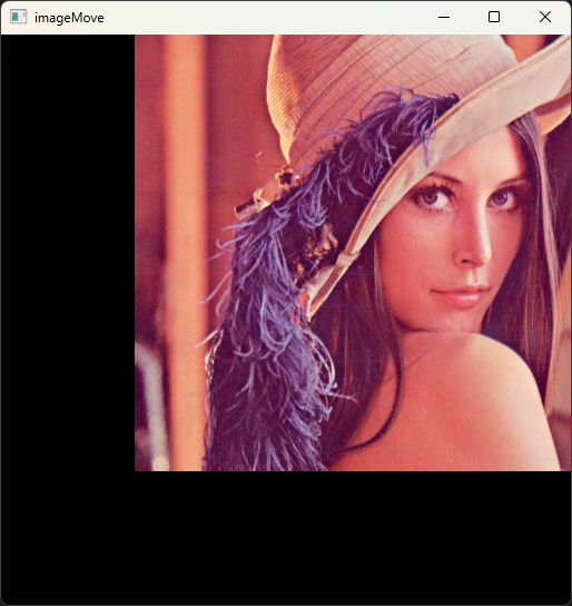
平移
平移是对象位置的移动。如果我们想要将\((x,y)\) 偏移至并\((tx,t_y)\),我们可以创建转换矩阵\(M\)如下:
\[
M =
\begin{bmatrix}
1 & 0 & t_x \\
0 & 1 & t_y
\end{bmatrix}
\]
当想将原始图像向右上移动120个像素时,矩阵\(M\)可以为:
\[
M =
\begin{bmatrix}
1 & 0 & 120 \\
0 & 1 & -120
\end{bmatrix}
\]
例如:
1
2
3
4
5
6
7
8
9
10
| import cv2 as cv
import numpy as np
image = cv.imread("pic/lena.png")
h,w = image.shape[:2]
M = np.float32([[1, 0, 120], [0, 1, -120]])
imageMove = cv.warpAffine(image, M, (w, h))
cv.imshow("image", image)
cv.imshow("imageMove", imageMove)
cv.waitKey()
cv.destroyAllWindows()
|
 屏幕截图 2025-01-21
160629.png
屏幕截图 2025-01-21
160629.png
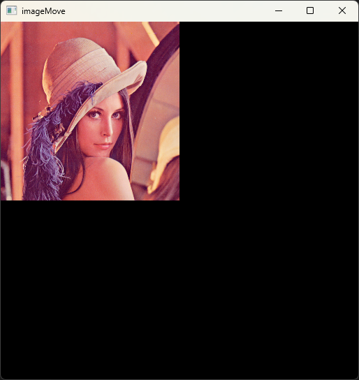
缩放
当想将原始图像缩小为一半时,矩阵\(M\)可以为:
\[
M =
\begin{bmatrix}
0.5 & 0 & 0 \\
0 & 0.5 & 0
\end{bmatrix}
\]
例如:
1
2
3
4
5
6
7
8
9
10
| import cv2 as cv
import numpy as np
image = cv.imread("pic/lena.png")
h,w = image.shape[:2]
M = np.float32([[0.5, 0, 0], [0, 0.5, 0]])
imageMove = cv.warpAffine(image, M, (w, h))
cv.imshow("image", image)
cv.imshow("imageMove", imageMove)
cv.waitKey()
cv.destroyAllWindows()
|
 屏幕截图 2025-01-21
161030.png
屏幕截图 2025-01-21
161030.png
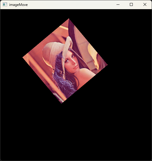
旋转
在OpenCV中,当进行旋转操作时,可以通过函数cv2.getRotationMatrix2D()得到仿射变换函数cv2.warpAffine()的转换矩阵。其一般格式为:
1
| ret = cv2. getRotationMatrix2D(center, angle,scale)
|
- center是旋转的中心点。
- angle表示旋转角度,正数为顺时针旋转,负数为逆时针旋转。
- scale表示变换尺度。
例如,要将图片缩小至原来的0.4后,逆时针旋转40°:
1
2
3
4
5
6
7
8
9
10
| import cv2 as cv
image = cv.imread("pic/lena.png")
h, w = image.shape[:2]
M = cv.getRotationMatrix2D((w/3, h/3), 40, 0.4)
imageMove = cv.warpAffine(image, M, (w, h))
cv.imshow("image", image)
cv.imshow("imageMove", imageMove)
cv.waitKey()
cv.destroyAllWindows()
|
 屏幕截图 2025-01-21
162052.png
屏幕截图 2025-01-21
162052.png
重映射
将一幅图像内的像素点放置到另一幅图像的指定位置,这个操作过程叫作重映射。重映射通过修改像素点的位置得到一幅新图像。因此,在构建一幅新图像时,需要确定新图像中每个像素点与原始图像所对应的位置。所以,映射函数的作用就是查找新图像像素在原始图像内的位置。OpenCV中的cv2.remap()函数提供了十分方便的自定义重映射方式。其一般格式如下:
1
| dst = cv2. remap(src, map1, map2, interpolation[, borderMode[, borderValue]])
|
- dst表示目标图像。
- src表示原始的图像。
- map1表示点(x, y)的一个映射或者点(x, y)的x值。
- map2表示的值与map1有关。当map1表示点(x,
y)的一个映射时,map2为空;当map1表示点(x, y)的x值时,map2表示点(x,
y)的y值。
- interpolation表示插值方式。
- borderMode表示边界模式。
- borderValue表示边界值,默认为0。
注意
mapl和map2的值都是浮点数,所以目标图像可以映射回一个非整数的值,这意味着目标图像可以映射到原始图像中不存在像素值的位置。此时,函数中的interpolation参数可以控制插值方式对图像进行插值操作。
复制
1
2
3
4
5
6
7
8
9
10
11
12
13
14
15
16
17
| import cv2 as cv
import numpy as np
image = np.random.randint(0, 256, size=[6, 6], dtype=np.uint8)
w, h = image.shape
x = np.zeros((w, h), np.float32)
y = np.zeros((w, h), np.float32)
for i in range(w):
for j in range(h):
x[(i, j)] = j
y[(i, j)] = i
rst = cv.remap(image, x, y, cv.INTER_LINEAR)
print("image=\n", image)
print("rst=\n", rst)
|
1
2
3
4
5
6
7
8
9
10
11
12
13
14
| image=
[[177 38 121 254 235 172]
[174 128 158 69 15 229]
[143 23 36 125 61 195]
[ 86 202 202 60 78 17]
[192 111 113 47 23 99]
[149 239 11 19 210 251]]
rst=
[[177 38 121 254 235 172]
[174 128 158 69 15 229]
[143 23 36 125 61 195]
[ 86 202 202 60 78 17]
[192 111 113 47 23 99]
[149 239 11 19 210 251]]
|
通过remap()函数实现图像的复制:
1
2
3
4
5
6
7
8
9
10
11
12
13
14
15
16
17
18
19
| import cv2 as cv
import numpy as np
image = cv.imread("pic/lena.png")
w, h = image.shape[:2]
map1 = np.zeros((w,h), np.float32)
map2 = np.zeros((w,h), np.float32)
for i in range(w):
for j in range(h):
map1[(i, j)] = j
map2[(i, j)] = i
rst = cv.remap(image, map1, map2, cv.INTER_LINEAR)
cv.imshow("image", image)
cv.imshow("rst", rst)
cv.waitKey()
cv.destroyAllWindows()
|
绕x轴旋转
图像绕着x轴翻转,在数学上是指映射过程中x坐标轴的值保持不变,y坐标轴的值以x轴为对称轴进行交换。使用remap()函数实现时,map1的值保持不变,map2的值设置为“总行数-1-当前行号”,这是由于OpenCV中行号的下标是从0开始决定的。
例如:
1
2
3
4
5
6
7
8
9
10
11
12
13
14
15
16
17
| import cv2 as cv
import numpy as np
image = np.random.randint(0, 256, size=[6, 6], dtype=np.uint8)
w, h = image.shape
x = np.zeros((w, h), np.float32)
y = np.zeros((w, h), np.float32)
for i in range(w):
for j in range(h):
x[(i, j)] = j
y[(i, j)] = w - 1- i
rst = cv.remap(image, x, y, cv.INTER_LINEAR)
print("image=\n", image)
print("rst=\n", rst)
|
1
2
3
4
5
6
7
8
9
10
11
12
13
14
| image=
[[204 212 30 213 107 247]
[103 121 174 81 214 247]
[218 203 119 69 170 143]
[ 18 151 183 0 0 126]
[ 89 170 103 69 161 118]
[229 176 62 240 99 33]]
rst=
[[229 176 62 240 99 33]
[ 89 170 103 69 161 118]
[ 18 151 183 0 0 126]
[218 203 119 69 170 143]
[103 121 174 81 214 247]
[204 212 30 213 107 247]]
|
绕y轴旋转
图像绕着y轴翻转,在数学上是指映射过程中y坐标轴的值保持不变,x坐标轴的值以y轴为对称轴进行交换。使用remap()函数实现时,map2的值保持不变,map1的值设置为“总列数-1-当前列号”,这是由于OpenCV中列号的下标是从0开始决定的。
例如:
1
2
3
4
5
6
7
8
9
10
11
12
13
14
15
16
17
| import cv2 as cv
import numpy as np
image = np.random.randint(0, 256, size=[6, 6], dtype=np.uint8)
w, h = image.shape
x = np.zeros((w, h), np.float32)
y = np.zeros((w, h), np.float32)
for i in range(w):
for j in range(h):
x[(i, j)] = h - 1 - j
y[(i, j)] = i
rst = cv.remap(image, x, y, cv.INTER_LINEAR)
print("image=\n", image)
print("rst=\n", rst)
|
1
2
3
4
5
6
7
8
9
10
11
12
13
14
| image=
[[182 211 25 119 17 24]
[ 60 42 209 135 122 240]
[ 25 19 225 67 112 18]
[ 73 35 238 205 189 141]
[249 179 11 129 115 138]
[200 44 174 13 34 2]]
rst=
[[ 24 17 119 25 211 182]
[240 122 135 209 42 60]
[ 18 112 67 225 19 25]
[141 189 205 238 35 73]
[138 115 129 11 179 249]
[ 2 34 13 174 44 200]]
|
绕x轴和y轴旋转
图像绕着x轴、y轴翻转,在数学上是指映射过程中,x坐标轴的值以y轴为对称轴进行交换,y坐标轴的值以x轴为对称轴进行交换。使用remap()函数实现时,map1的值设置为“总行数-1-当前行号”,map2的值设置为“总列数-1-当前列号”,这是由于OpenCV中行列号的下标是从0开始决定的。
1
2
3
4
5
6
7
8
9
10
11
12
13
14
15
16
17
| import cv2 as cv
import numpy as np
image = np.random.randint(0, 256, size=[6, 6], dtype=np.uint8)
w, h = image.shape
x = np.zeros((w, h), np.float32)
y = np.zeros((w, h), np.float32)
for i in range(w):
for j in range(h):
x[(i, j)] = h - 1 - j
y[(i, j)] = w - 1 - i
rst = cv.remap(image, x, y, cv.INTER_LINEAR)
print("image=\n", image)
print("rst=\n", rst)
|
1
2
3
4
5
6
7
8
9
10
11
12
13
14
| image=
[[ 81 44 137 186 35 194]
[ 3 140 26 23 142 158]
[237 155 158 90 173 11]
[ 71 92 62 55 155 1]
[175 218 234 63 240 34]
[ 68 101 148 160 123 177]]
rst=
[[177 123 160 148 101 68]
[ 34 240 63 234 218 175]
[ 1 155 55 62 92 71]
[ 11 173 90 158 155 237]
[158 142 23 26 140 3]
[194 35 186 137 44 81]]
|
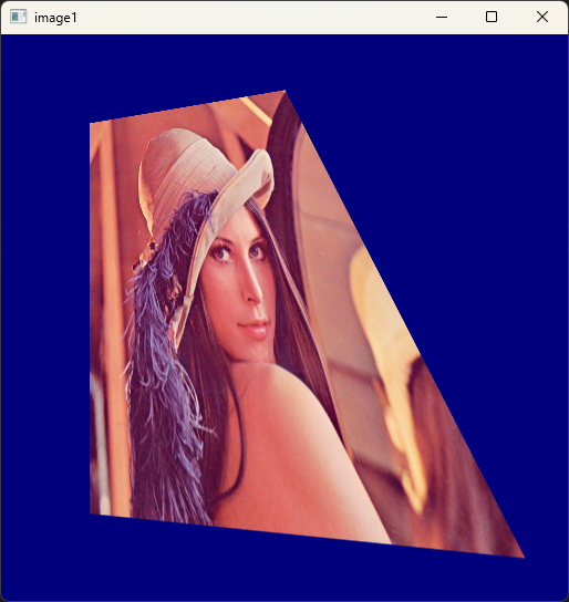
投影变换
在仿射变换的过程中,物体的转换都是在二维空间中完成的,但是如果物体在三维空间中发生了转换,这种转换一般叫作投影变换。
原理简介
因为投影变换是在三维空间内进行的,所以对其进行修正十分困难。但是如果物体是平面的,那么就能通过二维投影变换对此物体三维变换进行模型化,这就是专用的二维投影变换,可由如下公式描述:
$$
\[\begin{pmatrix}
\widetilde{x} \\
\widetilde{y} \\
\widetilde{z}
\end{pmatrix}\]
=
\[\begin{pmatrix}
a_{11} & a_{12} & a_{13} \\
a_{21} & a_{22} & a_{23} \\
a_{31} & a_{32} & a_{33}
\end{pmatrix}\]
\[\begin{pmatrix}
x \\
y \\
z
\end{pmatrix}\]
$$
在OpenCV中提供了cv2.getPerspectiveTransform()函数来计算投影变换矩阵,其一般格式为:
1
| cv2.getPerspectiveTransform(src,dst)
|
注意
这里需要输入4组对应的坐标变换,src和dst分别是4×2的二维矩阵,其中每一行代表一个坐标,而且数据类型必须是32位浮点型,否则会报错。
Python实现
类似于仿射变换,OpenCV提供了cv2.warpPerspective()函数来实现投影变换功能,其一般格式为:
1
| cv2.warpPerspective(src,M,dsize[,dst[,flags[,borderMode[,borderValue]]]])
|
- src表示原始的图像。
- M表示投影变换矩阵。
- dsize表示投影后图像的大小。
- flags表示插值方式。
- borderMode表示边界模式。
- borderValue表示边界值。
其使用方法与仿射变换相似,只是输入的变换矩阵变为3行3列的投影变换矩阵。
1
2
3
4
5
6
7
8
9
10
11
12
13
14
15
16
17
| import cv2 as cv
import numpy as np
image = cv.imread("pic/lena.png")
h, w = image.shape[:2]
src = np.array([[0, 0], [w - 1, 0], [0, h - 1], [w - 1, h - 1]], np.float32)
dst = np.array([[80, 80], [w/2, 50], [80, h - 80], [w - 40, h - 40]], np.float32)
M = cv.getPerspectiveTransform(src, dst)
image1 = cv.warpPerspective(image, M, (w, h), borderValue=125)
cv.imshow("image", image)
cv.imshow("image1", image1)
cv.waitKey()
cv.destroyAllWindows()
|
 屏幕截图 2025-01-21
172342.png
屏幕截图 2025-01-21
172342.png
极坐标变换
原理简介
笛卡尔坐标转极坐标
笛卡尔坐标系上\(xOy\)上任意一点\((x, y)\),以\((\bar{x},
\bar{y})\)为中心,通过以下计算公式对应到极坐标系\(\theta o r\):
\[
\begin{align}
r = \sqrt{(x - \bar{x})^2 + (y - \bar{y})^2}, \\
\theta =
\begin{cases}
2{\rm \pi} & y - \bar{y} \leq 0, \\
\arctan2(x - \bar{x}, y - \bar{y}) & y - \bar{y} > 0. \\
\end{cases}
\end{align}
\]
上式中,θ的取值范围用角度表示为0~360°,反正切函数\(\arctan2\)返回的角度和笛卡儿坐标点所在的象限有关,如果\((x - \bar{x}, y -
\bar{y})\)在第一象限,反正切的角度范围为0~90°;如果在第二象限,反正切的角度范围为90°~180°;如果在第三象限,反正切的角度范围为-180°~-90°;如果在第四象限,反正切的角度范围为-90°~0°。通常将\(y - \bar{y} \leq
0\)时返回的正切角度加上一个周期360°,所以经过极坐标变换后的角度范围为0~360°。
极坐标转笛卡尔坐标
在已知极坐标\((\theta,
r)\)和笛卡尔坐标\((\bar{x},
\bar{y})\)的条件下,计算笛卡尔坐标\((x,
y)\)以\((\bar{x},
\bar{y})\)为中心的极坐标变换是\((\theta, r)\),可通过一下公式计算:
\[
\begin{align}
x = \bar{x} + r\cos\theta, \\
y = \bar{y} + r\sin\theta.
\end{align}
\]
Python实现
在OpenCV中提供了两种进行极坐标变换的函数,分别是linearPolar()函数和logPolar()函数,其中linearPolar()函数的一般格式为:
1
| cv2.linearPolar(src, dst, center, maxRadius, flags)
|
- src表示原始的图像。
- dst表示输出图像。
- center表示极坐标变换中心。
- maxRadius表示极坐标变换的最大距离。
- flags表示插值算法。
logPolar()函数的一般格式为:
1
| cv2.logPolar(src, dst, center, M, flags)
|
- src表示原始的图像。
- dst表示输出图像。
- center表示极坐标变换中心。
- M表示极坐标变换的系数。
- flags表示转换的方向。
例如,使用linearPolar():
1
2
3
4
5
6
7
8
9
10
| import cv2 as cv
image = cv.imread("pic/circles.png", cv.IMREAD_ANYCOLOR)
dst = cv.linearPolar(image, (251, 249), 225, cv.INTER_LINEAR)
cv.imshow("image", image)
cv.imshow("dst", dst)
cv.waitKey()
cv.destroyAllWindows()
|
使用logPolar():
1
2
3
4
5
6
7
8
9
10
11
12
13
14
15
16
17
18
| import cv2 as cv
image = cv.imread("pic/circles.png", cv.IMREAD_ANYCOLOR)
M1 = 20
M2 = 50
M3 = 90
dst1 = cv.logPolar(image, (251, 249), M1, cv.WARP_FILL_OUTLIERS)
dst2 = cv.logPolar(image, (251, 249), M2, cv.WARP_FILL_OUTLIERS)
dst3 = cv.logPolar(image, (251, 249), M3, cv.WARP_FILL_OUTLIERS)
cv.imshow("image", image)
cv.imshow("dst1", dst1)
cv.imshow("dst2", dst2)
cv.imshow("dst3", dst3)
cv.waitKey()
cv.destroyAllWindows()
|
